1. A little history and philosophy
Numbers and geometry are two fundamental topics from the beginning of mathematics. Thanks to genius René Descartes, one of the greatest philosophers and mathematicians in the 17th century, who invented coordinate geometry (analytical geometry), a solid bridge was established between numbers and geometry. Points are associated to a set of numbers called coordinates, lines and surfaces are to algebraic equations. It seems that Cartesian coordinate system provides a very powerful tool to handle geometric objects and describe transformations. And indeed the idea of coordinate system has influenced the whole math, including the discovery of differential calculus by Newton and Leibniz regarding derivative (algebraic quantity) as the slope of tangent line (geometric quantity), and the emergence of differential geometry of curves and surfaces (geometric object), which can be described by parameterized smooth mappings (algebraic object).
Unfortunately, one has to admit that a lot of computational complexities result from interlude of numbers, which is really costly. In geometry, we mainly concern three aspects: 1. geometric objects themselves, such as shape, size (length, area, volume), angle etc.; 2. relationships between them like intersection, disjoint; 3. transformations, say stretch and contraction, reflection and rotation, also projection and rejection. We find actually all these aspects are independent with coordinate. What does that mean? That means no matter how coordinate system is chosen, these properties are invariant. In this sense, position and orientation of coordinate system doesn’t matter. Coordinate system being either skew or orthogonal, either scaled or normal, has no effect nothing about what we care. Hence a proper coordinate system is anticipated to facilitate the computation, though it is usually hard to get one or even impossible to have one in most cases.
Persons imbedded in Cartesian philosophy may devote their whole energy to finding methods of choosing a good coordinate system. And certainly, there are ones who do not, expecting to describe geometry without coordinate, or more specifically, coordinate-free geometry. Like Josiah Willard Gibbs, another great scientist making indispensable contributions to mathematical physics in the 19th century, found out multiplication of vectors, say dot product and cross product, has interesting geometric interpretations and formally gave them proper notations, which now is well known as part of vector analysis.
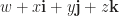
Actually, J.W. Gibbs is not the first to discovery an algebra for coordinate-free geometry. William Rowan Hamilton generalized complex number when he walked around Royal Canal in Dublin, Ireland after several years’ thinking, a shape of quaternion emerged into his mind. Then he could not resist his excitement and immediately carved the famous quaternion formula into the stone of Broom Bridge. Quaternion describes rotations in 3 dimension quite well. Inspired by W.R. Hamilton, many algebras such as bicomplex, hypercomplex, biquaternion have been come up with soon, all are associated distinct geometric pictures.
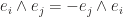
At almost meantime, Herrmann Günther Grassmann, German mathematician, the inventor of multilinear algebra, suggested exterior product in replace of cross product to achieve (multi)vector multiplications in higher dimension. In Grassmann algebra, a p-dimensional object is denoted as a p-vector, associated with magnitude and direction(orientation). For example, 1-vector is as usual a line segment. 2-vector (or bivector) is an area element, with magnitude as the area and direction as the plane which it lies, instead of normal vector in Gibbs’ vector algebra.
Grassmann algebra (also known as exterior algebra) is good enough to answer a lot of geometric questions since it can describe higher dimensional object. But William Kingdon Clifford, mathematician and philosopher, hoped for a unified algebraic framework incorporating all above number systems. His research on extensive Grassmann algebra led him to geometric algebra, which is part of Clifford algebra focusing more on theoretical, rather than geometric aspect. Clifford algebra then offers many great insights in both mathematics and theoretical physics. But it seems its geometric interpretation was forgot by people. Until late 20th century when David Hestenes rediscovery it, geometric algebra resuscitate to apply in more areas than fundamental physics, including image processing and robotics. D. Hestnes said, “geometry without algebra is dumb, algebra without geometry is blind.”
We will in the following briefly look at geometric algebra, hoping for an interesting journey.
2. Inspiration for geometric algebra
Let’s see what happens if multiply two vectors in 


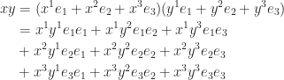
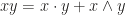
To endow the product with geometric meaning, we wish to have 
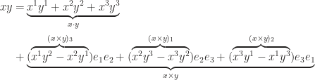
It’s readily seen that the product, composing of dot product and cross product, also applies to 2 dimensional case. Readers may find out that we add a non-scalar 


Note we also have

Equipped with wedge product, we can try to compute triple product with 
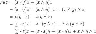
The geometric image shows that the sum of any two of the first three terms is perpendicular to the third, and the volume of parallelepiped equals the magnitude of the last term. Similarly, it’s readily to show (show it)

3. Some jargons and formulae
Since now we have a first touch on geometric algebra, it’s time to formally describe it. Yes, we don’t define it in this post because it obscures the visual image. Basically a geometric algebra of dimension 


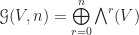
Evidently, a multivector 
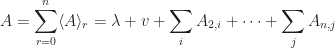
where 


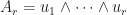


The first part of the product is called inner product and the second part outer product, defined as the following,

Note that we don’t mention basis, hence coordinate of vector, at all, which embody the property of coordinate-free of geometric algebra.
4. Properties of geometric algebra
We will list a collection of properties in geometric algebra. Readers will see that each property is supported by geometric fact which is very intuitive. By convention, we use lower letters to denote vectors and upper letters for blades.


For the limitedness of time, I have to omit the proof and explanation for now. I will make it up in a few days. As we can have seen, inner product with a vector contracts the subspace to one perpendicular to it, while outer product with a vector extends the subspace to one containing it. It is should be emphasized that geometric product can be defined on any two multivectors, which we will discuss it in the following post. Geometric product itself doesn’t have clear geometric insight, yet it collects different geometric facts together.
 etc, and element of a field
  , called scalar (or number), is denoted by
  etc.
etc.

 s.t.
s.t.  for each
 s.t.
s.t. 
 , where 1 is multiplicative identity of

 into the definition to display a very implicit yet natural identification between scalar multiplication from the left side and the right side, namely we don’t distinguish
  , letting
  ,
,  constructs a contradiction. As we have seen, even the most natural identification may fail when a simple condition doesn’t hold. We should be careful with every intuition before it is rigorously verified from axioms and established theorems. We will encounter many more natural identifications in the following sections, in which readers may gradually feel how unreliable the intuition is.
 can be viewed as an arrow starting from the initial point of vector
  and terminating at the end point of vector
  be the collection of linearly independent subsets. We furnish
  ,
,  is apparently an upper bound of
  . We shall require
  for applying Zorn’s lemma, that is, vectors in
  are linear independent. To this end, observe that for any finite subsets of vectors
  , there is an element of the chain
  such that
  for all
  . But
. But  is linearly independent set, so is
  . By Zorn’s lemma, there exists (at least) a maximal element
  . We claim
  . We have
  be linearly independent and hence belongs to
  .
. 
 , we can associate a unique coordinate
  as identificator under a specific set of basis vectors
  , and write
  (Here we adopt
  with respect to a new set of basis
  , where
  is the transformation matrix, namely
  . In such basis, vector
  . Since vector itself doesn’t change with basis (change of basis is essentially
 , or
, or
 is the inverse of
  . We find that coordinate of vector changes inversely to transformation law of change of basis. So in general, we speak of vector referring to contravariant vector.
 for each vector
  , called dual space of
  such that
  , namely the inverse of basis matrix
  . A dual vector
  then can be written as
  . If we change basis from
  , letting
  , we still have
 is inverse matrix of change of basis and
  . Then,
 , equivalently,
 be an open set, on which a vector field
  is defined. Suppose
  is a differentiable function with
  , then we have
 is identified with the gradient of
 and we multiply them formally, denoted by
  .
.
 , then the expression reduces to
 , there is a natural identification relation,
 be hodge star operator mapping between vector and pseudovector (
 ) space, then
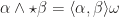
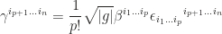
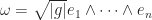 be
be  be determinant of metric matrix. We can use this identity to compute any hodge dual, even for each
  . Suppose
 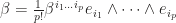 and
and  , take
 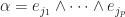 , then
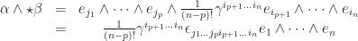


 , then
 is the signature of metric. This identification by Hodge dual, though looks complicated for computation, is natural just like turn a ladder upside down, The first stage becomes the last and vice versa. Because of the basis-independent property of Levi-Civita symbol in Hodge dual, for every improper rotation, pseudovectors gain a minus sign. That’s why bivector, hence the angular momentum, doesn’t belong to contravariant or covariant vector!
 introduced by Albert Einstein in 1916. For example, given two vectors
  , we write the inner product
 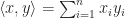 as in new notation
  . At the first glance there is nothing special as just omit the summation notation (This is exactly what I feel when I first saw the notation). But I will show you this reduction brings much more than convenience. Moreover, it indicates the object which the component belongs to. Specifically speaking, it distinguishes the type of the
  and matrices of proper dimensions by capital letters
  .
.


 .
. is equivalent to
  , but not to
  . As for non-repeated indices, they appear at the same time on both sides of the identity, and at the same position, both in upper or both in lower positions. Note that both superscript and subscript are indices rather than powers. Say, we always use
  to denote the second component of vector
  rather than


 naturally equates from the above identities, where
  means inner product with respect to
  means inner product of matrices. Till now, we are able to summarize and formally state the following.
 is an indicating function of identification of two indices.
![\delta_{ij}=\delta^i_j=\delta^{ij}=[i=j]=\begin{cases} 1& \text{if } i=j \\ 0 & \text{if } i \neq j\end{cases}](https://s0.wp.com/latex.php?latex=%5Cdelta_%7Bij%7D%3D%5Cdelta%5Ei_j%3D%5Cdelta%5E%7Bij%7D%3D%5Bi%3Dj%5D%3D%5Cbegin%7Bcases%7D+1%26+%5Ctext%7Bif+%7D+i%3Dj+%5C%5C+0+%26+%5Ctext%7Bif+%7D+i+%5Cneq+j%5Cend%7Bcases%7D&bg=ffffff&fg=1e1c1b&s=0&c=20201002)
![[\cdot]](https://s0.wp.com/latex.php?latex=%5B%5Ccdot%5D&bg=ffffff&fg=1e1c1b&s=0&c=20201002) is
is  holds and 0 otherwise. Kronecker delta looks like identity matrix and plays role of replacing index. For example,
  leaving
  by
by  . And
. And  not only replaces the index, but also pulls down superscript, which can be seen as transpose of the vector. Note that
  , where
  is defined as the
  , equivalently,
  where
where  is the parity of
  , the number of inversions in
  are the same.
 , where
  is
is  terms contained in summation, only those terms having
  , we find that
  . Surprising, right? As for a direct application in vector algebra, we have
  , considering the determinant rule for computing
 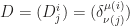 , where
  are permutations of order
  . According to the above,
![\delta^{\mu(i)}_{\nu(\sigma(j))}=[\mu(i)=\nu(\sigma(j))]=[\nu^{-1}(\mu(i))=\sigma(j)]=\delta^{\nu^{-1}(\mu(i))}_{\sigma(j)}](https://s0.wp.com/latex.php?latex=%5Cdelta%5E%7B%5Cmu%28i%29%7D_%7B%5Cnu%28%5Csigma%28j%29%29%7D%3D%5B%5Cmu%28i%29%3D%5Cnu%28%5Csigma%28j%29%29%5D%3D%5B%5Cnu%5E%7B-1%7D%28%5Cmu%28i%29%29%3D%5Csigma%28j%29%5D%3D%5Cdelta%5E%7B%5Cnu%5E%7B-1%7D%28%5Cmu%28i%29%29%7D_%7B%5Csigma%28j%29%7D&bg=ffffff&fg=1e1c1b&s=0&c=20201002) and
and 

 gives the sign of permutation
 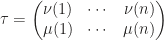 . Also, it’s readily to check
  whenever
  or
or  for some
  . The permutation
  is so common worthy a new symbol, called generalized Kronecker delta, defined as
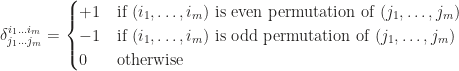
 doesn’t have to be
  , we have
  . When
  , the trick is to add dummy indices and consider
  . By definition, since the last
  indices are the same, we need only to consider the permutation of the rest
  copies of permutations of the rest indices. Therefore,
 . Let’s see what the role does generalized Kronecker delta play. It doesn’t simply replace the index any more, otherwise
 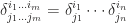 , which is obviously wrong. Let
 ![S^{i_1 \ldots i_m k_{m+1} \ldots k_n}=\delta^{i_1 \ldots i_m}_{j_1 \ldots j_m}T^{j_1 \ldots j_m k_{m+1} \ldots k_n}=m!T^{[i_1 \ldots i_m] k_{m+1} \ldots k_n}](https://s0.wp.com/latex.php?latex=S%5E%7Bi_1+%5Cldots+i_m+k_%7Bm%2B1%7D+%5Cldots+k_n%7D%3D%5Cdelta%5E%7Bi_1+%5Cldots+i_m%7D_%7Bj_1+%5Cldots+j_m%7DT%5E%7Bj_1+%5Cldots+j_m+k_%7Bm%2B1%7D+%5Cldots+k_n%7D%3Dm%21T%5E%7B%5Bi_1+%5Cldots+i_m%5D+k_%7Bm%2B1%7D+%5Cldots+k_n%7D&bg=ffffff&fg=1e1c1b&s=0&c=20201002) , where
, where ![T^{[i_1 \ldots i_m] k_{m+1} \ldots k_n}=\frac{1}{m!}\sum_{\sigma\in\mathscr{S}(m)}\mathop{sgn}(\sigma) T^{\sigma(i_1) \ldots \sigma(i_m) k_{m+1} \ldots k_n}](https://s0.wp.com/latex.php?latex=T%5E%7B%5Bi_1+%5Cldots+i_m%5D+k_%7Bm%2B1%7D+%5Cldots+k_n%7D%3D%5Cfrac%7B1%7D%7Bm%21%7D%5Csum_%7B%5Csigma%5Cin%5Cmathscr%7BS%7D%28m%29%7D%5Cmathop%7Bsgn%7D%28%5Csigma%29+T%5E%7B%5Csigma%28i_1%29+%5Cldots+%5Csigma%28i_m%29+k_%7Bm%2B1%7D+%5Cldots+k_n%7D&bg=ffffff&fg=1e1c1b&s=0&c=20201002) . Note that
. Note that  alternates sign when interchange any two indices from
  , actually